Before: SOL reserve = 30, Token reserve = 1,073,000,000
After:  SOL reserve = 31, Token reserve = 30 × 1,073,000,000 / 31 ≈ 1,038,387,097

Tokens received = 1,073,000,000 - 1,038,387,097 ≈ 34,612,903 tokens
Effective price = 1 SOL / 34,612,903 ≈ 0.0000000289 SOL per token
SOL reserve = 30 (virtual) + 85 (real) = 115
Token reserve = 30 × 1,073,000,000 / 115 ≈ 279,913,043 tokens remaining

Tokens sold during bonding curve = 1,073,000,000 - 279,913,043 ≈ 793,086,957 tokens
Graduation price ≈ 115 / 279,913,043 ≈ 0.000000411 SOL per token
Practical Applications for Traders
Calculating Your Entry's Upside Potential
Knowing where you are on the curve tells you how much upside remains before graduation:
- Entry at 5 SOL in curve: Graduation represents approximately a 10x from here
- Entry at 30 SOL in curve: Graduation represents approximately a 4x
- Entry at 60 SOL in curve: Graduation represents approximately a 2x
- Entry at 80 SOL in curve: Graduation represents approximately a 1.3x
This calculation helps you size positions appropriately. A 10x potential justifies more risk than a 1.3x potential.
Estimating Slippage Before Buying
Before executing a buy, calculate how many tokens you will actually receive at the current curve position:
Tokens received = Current token reserve - (k / (Current SOL reserve + Your buy amount))
If the estimated slippage exceeds your tolerance, reduce your buy size or set a limit order.
Trading frontends like Photon and BullX display estimated slippage before execution, but understanding the math lets you verify their calculations and plan multi-transaction strategies.
Identifying Curve Manipulation
Some deployers manipulate the bonding curve by:
- Buying a large portion at launch (through bundled transactions), pushing the price up rapidly, then selling to later buyers at inflated prices
- Creating artificial buy pressure with multiple wallets to attract organic buyers
- Timing sells at specific curve positions where their sell has maximum impact
By monitoring the SOL in the curve (visible on DEXScreener and Birdeye), you can estimate how much of the curve has been purchased by the deployer versus organic buyers.
Beyond Pump.fun: Other Bonding Curve Models
While Pump.fun dominates Solana token launches, other bonding curve implementations exist:
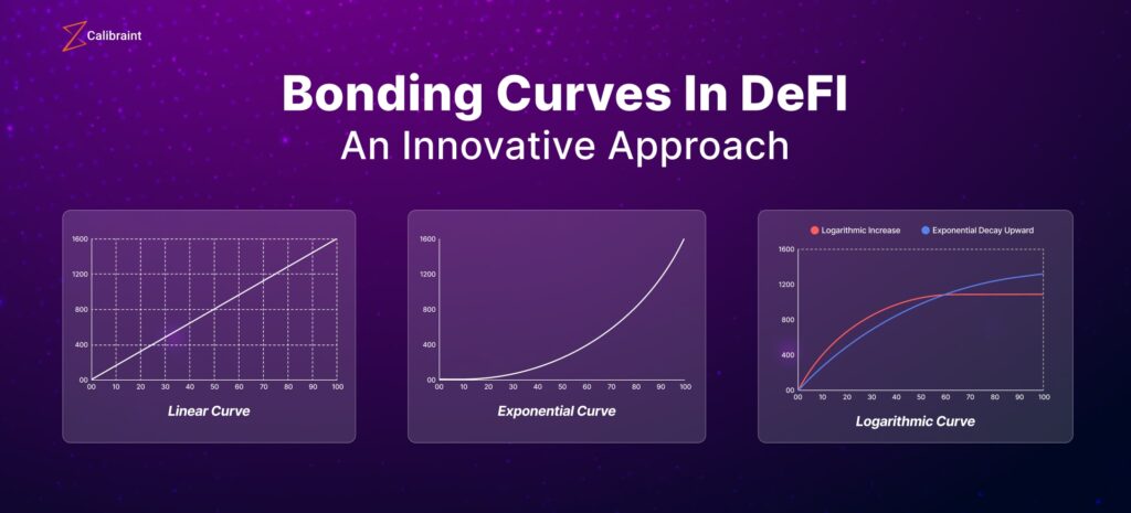
Linear Bonding Curves
Price increases linearly with supply: Price = a × Supply + b. These are simpler but less capital-efficient. Early buyers get a moderate advantage, but the price impact of large buys is more predictable.
Exponential Bonding Curves
Price increases exponentially: Price = a × e^(b × Supply). These create very steep price appreciation for early buyers. Even small increases in supply lead to dramatic price increases. Rarely used in practice because they make the token unaffordable very quickly.
Sigmoid Bonding Curves
Price follows an S-curve: slow growth initially, rapid growth in the middle, and tapering growth at the top. These are theoretically ideal for token distribution but more complex to implement and reason about.
Final Thoughts
Bonding curves are not just a technical implementation detail — they are the fundamental mechanism that determines token pricing for the majority of new Solana tokens. Understanding the math gives you a concrete edge: you can calculate exact returns at graduation, estimate slippage accurately, identify manipulation patterns, and make informed decisions about entry timing.
The next time you are evaluating a Pump.fun token, check how much SOL is in the curve before buying. That single number, combined with the math in this guide, tells you your potential upside to graduation, your expected slippage, and whether the curve has been heavily purchased by insiders.
Tools like DEXScreener, Birdeye, and RugCheck surface much of this data in user-friendly formats. But having the mathematical intuition behind what those numbers mean is what separates informed traders from those who are just following charts.
FAQ
Why does Pump.fun use virtual reserves instead of starting from zero?
Virtual reserves prevent the "first buyer gets infinite tokens" problem. Without virtual reserves, the first buy would get tokens at an effectively zero price with extreme slippage. Virtual SOL reserves create an artificial starting price that ensures even the first buyer pays a meaningful (though low) price. It also makes the price curve smoother for early trading, avoiding the extreme volatility that would occur at very low reserve levels.
Can the bonding curve parameters be changed after launch?
No. Once a token is created on Pump.fun, the bonding curve parameters (virtual reserves, graduation threshold) are fixed in the smart contract. The deployer cannot modify them. This is a feature — it means traders can trust that the pricing mechanics will not change mid-curve. However, different platforms may use different parameters for their bonding curves.
What happens to unsold tokens after graduation?
When a token graduates, the unsold tokens in the bonding curve (approximately 200-280 million tokens depending on how much was purchased) are deposited into the AMM pool alongside the accumulated SOL. These tokens form the sell-side liquidity in the pool. They are not burned or sent to the deployer — they become part of the tradeable liquidity.
Is it possible to predict which tokens will reach graduation?
Not with certainty, but you can identify factors that increase the probability: tokens from deployers with a history of graduations, tokens with organic (non-bundled) early buying, tokens with strong narratives or community backing, and tokens that attract attention from KOLs or social media. Tools like RugCheck and the Deployer Hunter on MadeOnSol help you evaluate deployer track records, which is one of the strongest predictive signals.